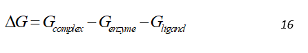
The MMPBSA [1,2] –a continuum/implicit solvation electrostatic methods– is the most rigorous of the approximate methods and has been the methods of choice for free energy calculations on a range of biological systems. A reasonably detailed physical model and fast computation (compared to ab initio methods) has led to its extensive usage. The MMPBSA method involves the calculation of absolute binding free energies by computing average free energies of the enzyme-inhibitor complex, and the free enzyme, inhibitor separately. These free energy values are then used to calculate the change in free energy by the following equation, which is average over an ensemble of frames from MD trajectories.
The solvent and counterions are removed from the MD trajectories and they are swapped by a continuum solvent representation in case the MD was performed with explicit solvent model and, a thermodynamic cycle is employed. The eventual objective of any free energy calculations method is the absolute free energy of binding in a solvent. However, in MD of solvated protein-ligand complex, most the energy contributions would come from solvent-solvent interactions, resulting in variations in total energy of an order of magnitude larger than the binding energy. Hence, direct calculations would require a very large number of snapshots to converge. The solution to this employed by MMPBSA is to use the thermodynamic cycle as shown in Figure 1. Where the binding free energy for system in vacuum is also calculated along with solvation energies of the complex, enzyme and ligand and the free energies for solvated system is given by:
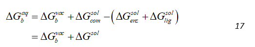
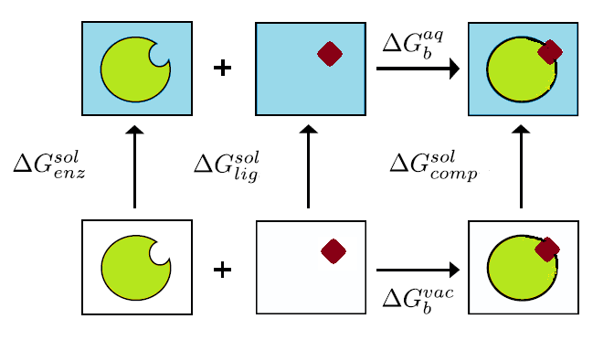
Figure 1: Thermodynamic cycle used in MMPBSA
The thermodynamic cycle used in to indirectly calculate the binding free energy in MMPBSA. The binding free energy changes in vacuo ( and the solvation free energies for the complex ( ), enzyme ) and ligand ) are calculated and then computed is computed by equation described above.
The and components of the binding free energies are calculated independently, using different methodologies. The free energies in vacuum , is calculated using the molecular mechanics, which can be decomposed into a sum of electrostatic, van der Waals and internal molecular mechanics interactions by Eq.18.
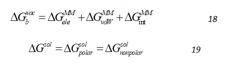
The term (solvation free energy) represents the free energy change associated with the movement of the solute from vacuum into a solvent environment. This can be decomposed into contributions from polar and non-polar interactions between the solute and solvent as:
The polar component of solvation energy is computed by numerically solving either linearized Poisson-Boltzmann or Generalized Born (MMGBSA) equation with an implicit solvent modeled as a high dielectric constant. The non-polar component is calculated using an empirical term related to the solvent accessible surface area.
Polar solvation energy using Poisson-Boltzmann (PB) equation
To compute the polar solvation energy ( ), it is required to model the electrostatic potential surrounding the system in an appropriate solvent. The Poisson-Boltzmann equation uses a continuum implicit solvent model with high dielectric constant, aqueous ions as a “diffuse charge cloud” and the solute as a collection of fixed point charges implanted in a lower dielectric continuum. Although there are many statistical mechanics based derivation of the PB equation. It may be derived very easily from Poisson’s equation [3, 4] also. Electric potential (φ) for a given charge distribution (ρf) can be estimated by solving the Poisson equation, where φ(r) at a point r generated by a charge distribution ρf(r) in an environment of dielectric coefficient ε(r) (relative to the permittivity of free space, ε0) is given by:
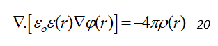
For the simulation of biomolecules, the functional form of ε(r) is subjected to the molecular geometry with the biomolecule represented as continuum region of low polarizability embedded in a surrounding continuum solvent of higher polarizability. For a biomolecular system, usually the dielectric constant of the solute is chosen to be in the range of 1 to 4 and a value of 80 is used to represent water.
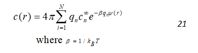
The charge distribution (ρf) comes from solute charge density (ρf(r)), and from the ions present in the solvent (c(r)). The ρf(r) can be defined as a set of delta functions centered on each solute atom’s center and scaled by the atom’s charge. The ion contribution is modeled as a continuum with charge distributed according to the Boltzmann distribution. For N ion species with charges qn and bulk concentrations of , the ion charge distribution is given by:
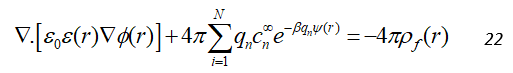
By combining the Eq. 20 and 21, we get the following equation:
In the case of an electrostatic neutral system, this can be simplified for two ions of equal bulk concentration, c , with opposite charges of equal magnitude, q as follows:
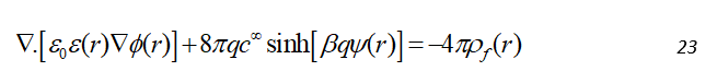
This equation can be rewritten in a linearized form by expanding the hyperbolic sine function as a Taylor series as:
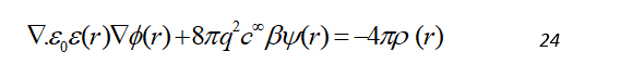
Eq. 24 is the linearized Poisson-Boltzmann equation, which can be solved by wide varieties of numerical methods. In MD packages, designed for simulation of biomolecules such as AMBER [5], the finite difference approach (FDM) is the most widely implemented method [6, 7]. A FDM comprises of succeeding steps of: (1) mapping atomic charges to the FD grid points; (2) assigning non-periodic/periodic boundary conditions; and (3) applying a dielectric model to define the high-dielectric (i.e., water) and low-dielectric (i.e., solute interior) regions and mapping it to the FD grid edges. These steps permit the partial differential equation to be transformed into a linear or nonlinear system. More details could be found in section 5.1.1 of AMBER14 manual [8].
References:
1. Sitkoff, D., K.A. Sharp, and B. Honig, Accurate Calculation of Hydration Free Energies Using Macroscopic Solvent Models. The Journal of Physical Chemistry, 1994. 98(7): p. 1978-1988.
2. Kollman, P.A., et al., Calculating Structures and Free Energies of Complex Molecules: Combining Molecular Mechanics and Continuum Models. Accounts of Chemical Research, 2000. 33(12): p. 889-897.
3. Dong, F., B. Olsen, and N.A. Baker, Computational Methods for Biomolecular Electrostatics. 2008. 84: p. 843-870.
4. Gilson, M.K. and B.H. Honig, The dielectric constant of a folded protein. Biopolymers, 1986. 25(11): p. 2097-2119.
5. D.A. Case, T.A.D., T.E. Cheatham, III, C.L. Simmerling, J. Wang, R.E. Duke, R., et al., AMBER 12. University of California, San Francisco., 2012.
6. Baker, N.A., Poisson–Boltzmann Methods for Biomolecular Electrostatics. 2004. 383: p. 94-118.
7. Fogolari, F., et al., Biomolecular Electrostatics with the Linearized Poisson-Boltzmann Equation. Biophysical Journal, 1999. 76(1): p. 1-16.
8. Amber 14 Reference Manual. 2014.
